This page is a demonstration of a ggplot graph rendered in Quarto.
library(tidyverse)
library(scales)
oews_pct <- read_rds("data/oews_pct.rds")
ggplot(oews_pct,
aes(x = pct_change,
y = wage,
fill = wage)) +
geom_col() +
geom_text(aes(label = label_percent(accuracy = 0.1)(pct_change),
color = wage),
nudge_x = 0.01) +
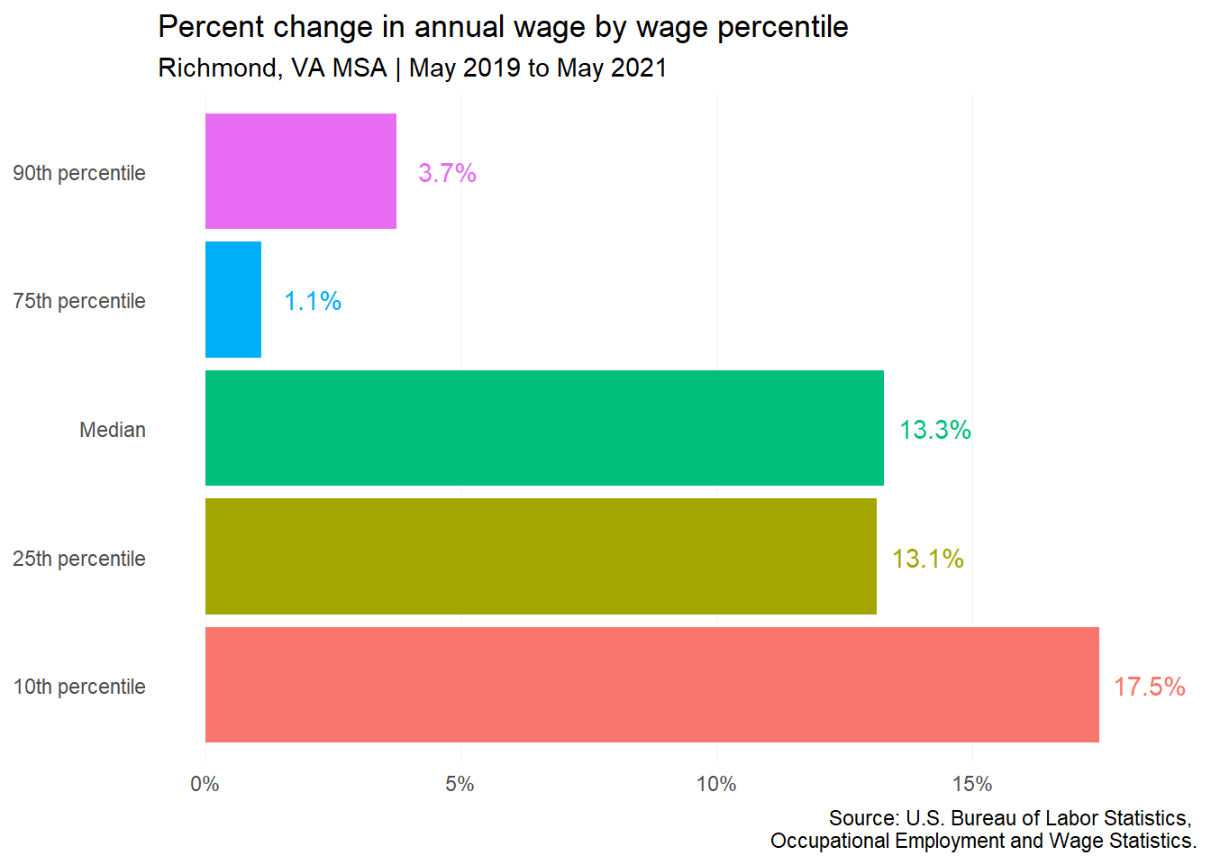
labs(title = "Percent change in annual wage by wage percentile",
subtitle = "Richmond, VA MSA | May 2019 to May 2021",
caption = "Source: U.S. Bureau of Labor Statistics,
Occupational Employment and Wage Statistics.") +
scale_x_continuous(labels = label_percent()) +
theme(axis.title = element_blank(),
axis.ticks = element_blank(),
panel.background = element_blank(),
panel.grid.major.y = element_blank(),
legend.position = "none",
panel.grid.major.x = element_line(color = "grey95",
size = 0.05))